GIS, predictive modelling, erosion, site monitoring

by David Ebert & Matthew Singer

Abstract
1.0 Introduction
1.1 The Study Area
2.0 Archaeological Predictive Modelling
2.1 Model Types
3.0 Erosion
4.0 Methodology
4.1 Predictive Modeling Methodology
4.2 Erosion Modelling Methodology
4.3 Monitoring Model
5.0 Project Improvements
5.1 APM Improvements
5.2 Erosion Model Improvements
6.0 Conclusions
Acknowledgements
Bibliography

 Abstract

This paper examines predictive modelling of two separate items of archaeological interest. First, the paper examines traditional archaeological predictive modelling of site location using environmental data. Archaeologists use predictive modelling in order to evaluate the potential for the occurrence of archaeological (or heritage) resources in areas that have not been investigated. Most commonly, this is done by using the known archaeological sites of a given region in a manner analogous to a training set in remote sensing image classification. Sites are statistically correlated against features of the modern environment (proxy variables) to determine the correlation of these environmental variables with site location. Ultimately, an environmental profile of sites is built with these correlations. A GIS was used to discover areas matching this environmental profile in areas that remain unsurveyed for archaeological resources. The result of this model was a map of archaeological potential for the occurrence of sites in a given area. Second, the paper looks at the forces of erosion active in an area which works to uncover archaeological sites. Erosion is an important factor in archaeological investigations, as archaeologists often find sites at places where erosion has occurred, making eroded soils one of the most productive areas for archaeological investigation. Using ArcView, this project modelled the potential for erosion in the study area, based on physiographic information, producing a map of erosion potential. Finally the paper investigates how these two models might be combined into a single model, which can be used to monitor sites which are in danger of being eroded or in areas of high erosion where sites are also likely to occur.

 1.0 Introduction

Archaeologists rarely seek out sites in areas of high erosion. Unless a survey is planned for areas susceptible to high erosion, the discovery of sites will be left to chance. Unfortunately, because erosion is ongoing, this means that many sites can be lost before they are found. Since artefacts are only of use to archaeologists when they are in situ, anything eroded from its primary context holds little archaeological information.

In the light of these comments this paper demonstrates how a geographic information system (GIS) based on inductive modelling can be employed to create two models, one predicting archaeological potential and the other erosion potential. Through collating the information in these two maps, a third map is created, giving a suggested monitoring program for areas that are likely to contain archaeological sites which are also likely to suffer from the effects of erosion. While predictive modelling in archaeology plays an important role in saving archaeological sites from destruction through development, it is rarely used in a proactive manner to identify sites that may be threatened by natural disturbances. Therefore, this project seeks to examine an application of predictive modelling which will extend its current usage.

 1.1 The Study Area

The study area is located in the boreal forest ecozone of west-central Manitoba (Canada), near the community of Flin Flon, and is shown in Figure 1. The study area was selected due to the availability of data from another project on which one of the authors (DE) was doing some research.

Figure 1: Study Area Location

This part of Manitoba has been continuously inhabited over the last 6000 years following the retreat of the glaciers and the draining of Glacial Lake Agassiz (Buchner et al. 1983). The area was inhabited by hunter-gatherer groups, similar to those of plains groups to the south. However, the hunting and gathering economy was not focused on bison, which was uncommon in this region, but rather on locally available woodland species of the boreal forest (Buchner et al. 1983).

The local population used stone-tool technology, were nomadic and likely organized into small groups or bands (Buchner et al. 1983). They had access to a network of inter-connecting waterways, often characterized as 'highways', and are thought to have been highly mobile. The generalized pattern of the seasonal round, as ethnographically documented, suggests that people gathered in larger groups on the major lakes in the summer, and then moved in family or extended family-sized groups to smaller lakes in the winter (Larcombe 1994).

Boreal sites tend to be small, with very low artefact densities, suggesting that they were occupied only on a short-term basis. Sites generally have no diagnostic artefacts and no organic preservation due to soil chemistry. Additionally, sites are typified by an extreme conflation of cultural layers. Soils in the boreal forest as a whole tend to be poorly developed (Gardner 1981: 6), as pedogenesis is influenced by climatic conditions, as well as differences in drainage and the parent material (Scott 1995: 88). The low rate of pedogenesis means that soil layers, when present, tend to be thin, if at all existent. This is why artefacts tend to be mixed.

The study area is less developed than other areas of Manitoba. Most sites have been found on the lake margins, where recreational development has occurred, but much less is known about inland areas. The major cultural impacts on archaeological sites are forestry and recreational development. However, archaeological sites, which for the most part are located on the shores of small and large lakes which dominate the landscape, also face significant impact from natural erosion, especially wave erosion.

 2.0 Archaeological Predictive Modelling

Archaeological predictive modelling (APM) is defined as 'a technique, used to predict archaeological site locations in a region, on the basis of observed patterns, or, on assumptions about human behaviour' (Kamermans and Wansleeben 1999) The growth of this method in archaeology has been linked with the development of commercially available GIS packages. Generally, it is a method which predicts the location of sites in a given region of unknown archaeological resources. There are two types of APM - inductive and deductive. The inductive model is the most common type of APM, however deductive modelling is thought to be superior, as it offers an explanation of the process by which settlement occurs (Dalla Bona 1994).

APM has been critiqued along a number of lines, especially on the basis of environmental determinism and the limited ability to model human behaviour (e.g. see Gaffney and van Leusen 1995; Ebert 2000). While these critiques have varying degrees of validity, they cannot deny that APM has met with both great success as well as great popularity in locating some categories of archaeological sites in North American archaeology. Given its popularity and success, APM will not 'go away' and archaeologists should seek ways to improve and engage with APM rather than to dismiss it. However, archaeologists employing predictive modelling should also been aware of these criticisms and try to address them in their modelling practices. GIS is particularly strong in the representation, manipulation and analysis of data that can be spatially referenced and quantified. In other words, GIS requires a location and a measurement of some sort at that location. These data would include many varieties of environmental data (e.g. slope, aspect, water, soils, etc.) as well as locational data (e.g. sites, lithic resources, etc.). However, the representation of these data can be problematic as the GIS requires its representation as either a point, line or polygon. For example, most site databases in North America represent sites as point locations, when polygons might be more appropriate, although often more difficult to accurately portray. There are three main areas in which GIS can be considered lacking: cognitive representations, temporal analysis and three-dimensional analysis. Cognitive representations are often difficult in GIS, due to the requirement of concrete spatial location assignments. Often cognitive ideas can be represented in this way, but more often their representation as a point, line or polygon becomes difficult. Temporally, GIS cannot adequately represent and analyze data that changes over time. For archaeologists this problem means that analysis of culture change can be difficult. Additionally, the fact that GIS cannot be considered to be truly three-dimensional hinders the analysis of three-dimensional archaeological deposits. Given these limitations, GIS can still be a powerful tool for archaeological analysis, as long as it is employed in a manner consistent with its strengths and cognisant of its failings.

 2.1 Model Types

In an inductive APM, the locations of known archaeological sites are investigated for their locational pattern primarily in relation to environmental variables (Kvamme 1992: 20), although other variables, such as economic or social factors, have occasionally been employed. Inductive models have become, by far, the more popular of the two kinds of model, due to their relative ease of construction (Dalla Bona 1994). In a manner analogous to the use of a training set in classifying remotely sensed images, locations of known archaeological sites are used to create an environmental profile of site location. The GIS is then used to determine which areas in regions of unknown archaeological resources have similar profiles. The result is normally a map of archaeological potential, generally divided into classes, such as low, medium and high (Dalla Bona 1994). Since inductive models begin with the site location data, conclusions are based upon any biases that may have been present in the original data set (Dalla Bona 1994). While predictions for site locations may be accomplished without the use of a GIS, these models are often too simple. The adoption of GIS allows the archaeologist to conduct more sophisticated modelling of human land use.

Most inductive models use a small core of environmental variables as correlates of site location, including: slope, aspect and distance to water (Kvamme and Jochim 1989). These are often referred to as proxy variables, as they are being used in a generally correlative nature, rather than a deterministic nature. Some studies use other variables, such as soil type or vegetation type. Despite their non-deterministic nature, environmental variables are recognised as being important for choosing suitable habitation locations. In other words, the physical environment is an important factor in attempting to re-create human land use. For example, slope is presumed to be important, as settlements are generally located on level surfaces (Kvamme and Jochim 1989). Water availability is unquestionably a significant factor, both for drinking and transportation purposes (Kvamme and Jochim 1989). The aspect of a site can be used to understand how it is protected from wind and other weather, thus giving an indication of available shelter (Kvamme and Jochim 1989). However, these environmental factors do not help us to discriminate amongst the multitude of locations which could fit these basic criteria. One obvious failing of this approach is that it cannot account for cognitive factors, which would help explain why some areas are chosen, while others are not.

Deductive APM focuses on systemic decisions in order to understand locational behaviour, through the use of either a general theory of human behaviour or some a priori knowledge (Kohler and Parker 1986). While deductive models are thought to be superior to inductive models, as they explain why sites are located where they are, this type of model is very rare in the literature. This lack of usage is likely due to the fact that deductive models are seen to be difficult to operationalize (Kohler and Parker 1986).

 3.0 Erosion

Erosion and archaeology are very similar, in the sense that both remove ground surfaces exposing cultural materials. An important aim of this project is to predict where soil erosion occurs. When a soil erosion model is used in conjunction with an archaeological predictive model, a powerful tool is created through which the archaeologist can predict and locate exposed cultural remains. To create the erosion model, three types of erosion are examined. These include wave erosion, slope erosion, and soil erosion. These three factors provide enough information to ascertain potential high-risk soil erosion areas.

The potential for soil erosion relates to its structure and texture. The texture refers to the size of the particle while the structure refers to how the particles cling together. Once the texture and structure are identified, they can provide clues for the likelihood for erosion to occur. The soils found in the study area are mixtures of three substances: silt, clay and sand. Clay has the finest texture, while sand has the coarsest. Large particles are more susceptible to erosion, while smaller soil particles can be used as binding agents with other materials to create a stronger bond. Andre and Anderson (1961) suggest that potential for soil erosion depends upon the ratio between the amount of soil surface needing adhesion and the amount and quality of the clays and silts. Smerdon and Beasley (1959) argue that a higher percentage of clay or aggregating materials creates lower potential for erosion. The potential for erosion of loam, sandy loam and sandy parent material are judged based on these studies.

The erosion potential model is made up of spatial relationships where point specific information is important, and aspatial relationships where point specific information is unimportant. The soil model is an aspatial relationship, because the specific location of the soil is not the factor of interest, rather, its general potential for erosion is the factor of concern. On the other hand both the wave model and slope model was based on spatial relationships, since only in specific locations do waves and slopes intersect with possible human activity. The wave model looks at both wind direction and aspect. These two characteristics were combined and erosion potential was determined based on places where aspect and wind direction indicated a higher potential for wave action. The slope model was also based on spatial relationships: in this case slope was directly influenced by topography. The use of both spatial and aspatial relationships has helped in the creation of the total erosion model.

 4.0 Methodology

Methodologically, the creation of the APM discussed here follows traditional methods, especially those described in (Dalla Bona 1994). However, because there were no similar guides for creating the erosion model, a methodology that parallels the creation of the APM is preferred. The following sections describe the methodology for 1) creating the APM, 2) creating the erosion model and 3) creating the combined monitoring model.

 4.1 Predictive Modeling Methodology

Tolko Industries Ltd. provided data in a digital format for the research. This data included information on: 1) ecozones, 2) bedrock geology, 3) surficial geology, 4) prominent landforms, 5) soils, 6) vegetation type, 7) watersheds and 8) infrastructure. While some of this data was useful (i.e. the soils and geological information), some of the data was less so (i.e. the ecozones and watersheds data). Digitizing at the computer facilities at the Anthropology Lab, University of Manitoba, accommodated additional data requirements. The digitizing functions of the Arcview 3.1 software were the primary method of data capture.

A digital elevation model (DEM) forms the basis of much of the landscape analysis in APM (Dalla Bona 1994). To create a DEM, ArcView has the capability to calculate a continuous elevation surface through the use of triangulated irregular networks (TINs). A TIN is a lattice of triangles, which have three points of known elevation as vertices (Burrough 1986). A by-product of a TIN is the calculation of the slope and aspect of each of the triangles (Burrough 1986), although ArcView will calculate these data as separate map layers. Since their invention, TINs have proved to be valuable ways of representing the landscape. For the most part, they have become an industry standard for the creation of DEMs.

For this project an inductive model was chosen reflecting the study team's familiarity with inductive approaches and the availability of appropriate software. Once an inductive model had been decided upon, the approach and method of weighting had to be further determined. The determination of model components can be done through the statistical approach suggested by Kvamme (1990). In this method, the environmental variables of interest at the location of known archaeological sites are tested against the background environment as a whole to identify whether there are statistically significant differences between the distribution of sites against a particular environmental variable (Kvamme 1990). Layers of environmental data are stored in grids in the (GIS), which in the case of this project were laid on a 30 x 30m grid. Each grid cell receives a value for each environmental variable. The values for each of the environmental variables are recorded for known archaeological site locations. The values at these locations can then be compared, through the use of goodness-of-fit statistics, to the distribution of values for those variables across the entire grid. For this project, the Kolmogorov-Smirnov Goodness-of-Fit-Test is employed (Kvamme 1990). This test examines the goodness-of-fit of a single sample to a referent population, and is appropriate for continuously distributed data, such as environmental data (Kvamme 1990). The cumulative frequency of data is compared to determine the maximum difference (Dmax). This value is compared against a critical value (D), which is calculated by:

When the maximum difference exceeds the critical value, it is said that there is a statistically significant difference between the sample and the referent sample population (Kvamme 1990).

The number of cells in each class of environment is entered into the spreadsheet. The environmental variables investigated were slope, aspect, distance to water and surficial geology. Soils were also initially investigated but ultimately had to be abandoned due to data problems. The majority of all known archaeological sites fall into an 'unknown' soil type category. An example of the statistical testing and weighting of the variables is shown in Tables 1 (statistical testing) and 2 (weighting) for the variable 'aspect'.

Table 1: Statistical Testing for the Aspect Variable

In the 'sites' column of Table 1, each of the sites in the study area is classified according to its aspect. In this case, six sites are classified as being on a flat surface, eight as being on north-facing slopes, and so forth. This number is translated into a cumulative frequency, which is shown in the adjacent column in the table. Next, each of the 30 x 30m cells in the entire study area, or what Kvamme (1990) calls the 'background environment', are tabulated as to their classification, shown in the 'Cells in the Environment' column and also converted to a cumulative frequency. The two cumulative frequencies are subtracted to get the difference. The maximum difference, called Dmax in this test, is then selected in order to assess the statistical significance. Here, Dmax is 0.775, where there are only 9.5 percent of sites located on flat land, versus nearly 88 percent in the study area as a whole. This leads us to state that there is a significant difference in site location based on aspect. This testing can then be used to make weightings.

Table 2: Aspect Weightings

Since variable weightings can profoundly alter the outcome of the predictive model, this project attempted to create a methodology that was objective in assigning the category weightings. Each variable was assigned a 'category weighting' which was reflective of the magnitude of the difference, or Dmax, in the statistical testing for all variables. So the variable with the highest Dmax value would get the highest category weight, and the variable with the lowest Dmax, the lowest. In the case of weightings for the variable of 'aspect', as shown in Table 2, it had one of the higher Dmax values, so it received a category weighting of 5. Secondary weights also had to be created to represent the internal differences in the values that a variable could take. For example 'aspect' could have values of north, northeast, east, southeast, south, southwest, west, northwest and flat. Presumably each of these would be more or less attractive. In the case of 'aspect', most sites occurred in the south and southeast values, so they received the highest secondary weights. Northeast had the lowest number of sites, so it received the lowest secondary weighting. As a final step in the weighting process, the category weights were multiplied by the secondary weights in order to get the overall weight, which was assigned to each of the cells in the GIS. So all of the cells on flat land receive a weighting value of 15 (category weight of 5 times a secondary weighting of 3 for flat, resulting in a product of 15). This process was repeated for all of the category and secondary weights, resulting in weighted map layers.

Once variable weightings were determined, it was simply a matter of entering the weights into the tables of each of the environmental variables in ArcView and using the Map Calculator to add together the weights for all of the proxy variables. The resultant APM map is shown in Figure 2. The 'high', 'medium' and 'low' archaeological potential categories were determined by dividing the total range into three equal ranges.

Model testing can occur in two forums - the lab and the field. In the scope of this project, being that it is primarily a laboratory experiment, field testing was not possible, which affects the reliability of the results accordingly. Lab-based testing can occur through validation, or through the use of red flag models (Altschul 1990). Validation can occur in one of two ways: meeting internal criteria, or testing against a subsample of sites (Kohler and Parker 1986). In the case of a subsample of sites, a portion of the sites in the study area are not included in the initial formulation of the model, but are 'held back' as a testing sample. Presumably, if the model has properly assessed the correlations between sites and environmental variables, the subsample should fall into areas of high or medium potential (i.e. be correctly predicted). However, it may be more difficult to remove a subsample from consideration, if site numbers are low in the study area, or show a great deal of variability.

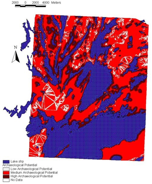
Figure 2: Archaeological Predictive Model

As shown in the model, the map actually shows too many areas of high and medium potential, and considerably fewer low potential areas. Normally, this would mean that the predictive model should be discarded. However, because this model was not to be employed by itself, the map was retained, to be later combined with the erosion models.

For this project, internal criteria were used for validation of the inductive model. In this case, a parallel procedure was used as in the statistical testing of variables. The numbers of cells in the environment in each of the potential categories (low, medium and high archaeological potential) can be compared to the number of sites in each of the potential categories using the Kolmogorov-Smirnov One-Sample Goodness-of-Fit statistical test. This test is shown in Table 3.

Table 3: Statistical Testing of the APM

Here, all of the sites used in the creation of the model fall into either high or medium potential. The Kolmogorov- Smirnov test then evaluates whether there is a statistically significant difference between the distribution of archaeological potential in the background environment versus the known archaeological sites' archaeological potential. In this case, Dmax is 0.476, allowing that there is a significant difference in archaeological potential for sites versus the background environment.

 4.2 Erosion Modelling Methodology

The slope of the ground surface affects the amount of erosion that may occur. The steeper the slope, the less time the soil has to absorb water, so more soil is lost due to runoff. Duley and Hays (1932) conclude that runoff increases rapidly from 0 to 3 percent slope and is slight for each additional percent. Soil loss increases slowly to 4 percent and increases rapidly after 7 percent slope. This model is the basis for classification of the slope erosion model.

Areas of slope greater than 7 percent are given a classification of high erosion potential. Areas of medium erosion potential include those places that have a slope from 4 to 7 percent. Lastly, areas of slope from 0 to 4 percent are low erosion potential areas. This information is combined with the wave erosion model to create the overall erosion potential map.

Wave or shore erosion is the loss of sediments from the shore area (Penner 1993: 9). Waves continually change and modify the shore zone. The wave erosion model is based upon wind direction and aspect. The lake size influences the size of the waves that reach the shore. Lake size combined with the aspect of an area can provide clues to locate areas of high potential for wave erosion. In Manitoba, there is generally a westerly wind blowing at a varying intensity. Large lakes have larger and more frequent wave action, while small lakes have smaller and less destructive waves. Separate themes in ArcView were created based on the size of the lake. The first theme is of lakes 1,000,000 ha and larger. The second theme is of lakes 500,000 ha to 1,000,000 ha and the last theme contained lakes 0 to 500,000 ha. Buffers of 20m were then created around each lake within each theme, and the new maps are labelled Small, Medium or Large Wave Erosion Zones. The 20m buffer is set to represent the areas that are susceptible to wave erosion. These maps are then changed to grid files so the map calculator can be used. Map Calculator is able to show exposed and unexposed areas in the erosion zone. Exposed areas are deemed to be those where large lake wave erosion and prevailing westerly winds are present. Exposed areas indicate high potential for erosion while unexposed areas have little potential. The wave erosion model is broken down into three different potentials for erosion. These are high, medium and low potentials, the criteria for which are shown in Table 4.

Table 4: Wave Erosion Model Potential Characteristics

Soil types depend on their place of origin and are dependent upon the type of parent material. The soil in our study area is made up of loam, sandy loam and sandy parent material. Loam is an equal mixture of silt, clay and sand, and is very fertile. Sandy loam includes more sand in the mixture and is more susceptible to erosion. Sandy parent material is the most susceptible to erosion because it contains the least amount of clay. Clay functions as a binding agent and helps the soil stay together during the erosion process (Leopold et al. 1964). Areas of erosion potential are thus dependent on the amount of clay in the soil. The validity of our soil erosion model is weak due to the fact that a large number of sites occurred in our unknown soil type area. Sandy parent material has the highest erosion potential, whereas sandy loam has a medium potential for erosion and loam has the lowest potential. Based on these classifications, a map was created and added to the total erosion model.

The combined erosion model is shown in Figure 3.

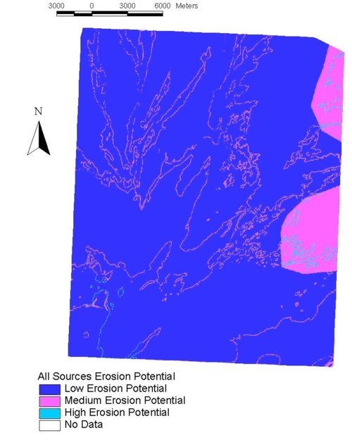
Figure 3: Combined Sources Erosion Model

 4.3 Monitoring Model

Once the models for erosion and archaeological potential were determined, it was necessary to establish a protocol by which monitoring priority could be assigned. Such a protocol was created through the use of a simple cross-tab table, shown in Table 5.

Table 5: Monitoring Model Priority Determination

Once the monitoring protocol was determined, the creation of a monitoring map was completed through the use of a series of Map Calculator queries to determine the areas falling into each of the groups. After each of these monitoring priority levels was determined, a field was added to each Map Calculator query, called Monitor Priority, and values of 1 (low monitor priority) to 3 (high monitor priority were assigned) and a single map created. This Monitoring priority model is shown in Figure 4.

There are clear areas of high, medium and low monitoring priority, despite the over-all high potential of the archaeological predictive model. Not surprisingly, the areas of high monitoring priority are on the western shores of the lakes, areas both of high archaeological potential and high erosion potential. While the model does not necessarily identify areas that would be surprising to field archaeologists, the creation of the monitoring model would help focus planning for archaeological projects in this region. This model would allow archaeologists to focus their work on specific areas that are

Figure 4: Monitoring Priority Zones

highest in their potential for erosion as well as containing archaeological sites. Any individuals involved in the protection of cultural resources, from government archaeologists to First Nations groups, could potentially benefit from this type of model.

 5.0 Project Improvements

There are few aspects of the laboratory project on which there could not be some improvement. In this section we draw attention to some improvements which offer ways to strengthen the overall model.

 5.1 APM Improvements

There are two areas of great concern with regards to the APM. First is the question of overall data quality. This concern revolves around the availability of intensively sampled data for the area before interpolation. This is of primary concern with the DEM. Second is the need for field testing of the model.

The DEM is cause for great concern, as the accuracy of the contour lines digitized from the 1:50,000 NTS maps are suspect. The NTS maps indicate few sample locations and any interpolation technique would be pushed to its limits of accuracy in creating contour intervals. Since the DEM is suspect, the derived data from the DEM, the slope and aspect maps, are also questionable. However, alternative sources of data are few. While the Government of Manitoba has covered much of the province with aerial photographs, suitable for elevation surveys by photogrammetry, the study area remains uncovered by the photographs. The concerns about data quality lead to concerns about error propagation. Since any errors in any of the inputs are not eliminated, they are perpetuated through each of the subsequent models, often creating new errors. In principle, data of the highest quality should always be employed. However, in this case while satisfactory to build the theoretical model, the data would ideally have been better.

Field-testing of APMs provides the highest level of test for the reliability of the model. While beyond the scope of this project, it would be of great utility to test the various zones of archaeological potential for the discovery of new sites. Through the data acquired from field-testing, a more rigorous evaluation and refinement of the model would be possible.

 5.2 Erosion Model Improvements

In addition to improving some of the data, such as the coverage of the soils data, the erosion model could have been improved through the addition of two important factors. One of those factors, vegetation, helps inhibit erosion, while the other, running water, is a powerful tool of erosion.

Vegetation can have numerous effects on soil. It would have been beneficial for this study to include identified areas of forest, grass cover and cultivation. These types of ground cover affect erosion through (Ayers 1936: 30):

1. direct dispersion of rain drops by leaves and shrubs.
2. creation of shielding by grasses and plants during rain storms.
3. creation of a binding system that holds the soil together.
4. introduction of new organic material into the soil which increases absorption and keeps the soil fertile for new growth.
5. keeping water levels even and therefore delaying the concentration in tributary drainage ways.
6. addition of air into the soil and humus which creates a more favourable environment for the creation of beneficial bacteria.

The best possible protection against erosion is a thick grouping of trees. Soils can be protected with a dense canopy, ground leaf litter and extensive tree root systems. This combination is also effective in areas with high slopes. Grass cover and crop cultivation varyingly effect erosion. Tilling exposes soils and leaves them vulnerable to wind erosion. In cultivation, the amount of time the soil is exposed without any crop cover will determine the amount of erosion that will occur. Factors such as roads and train tracks cause unnatural watersheds. Including these characteristics in our study area would have increased the possibility of identifying areas of high potential for erosion. These additional factors would have been included in this study, but there were no maps available at the time of initial examination.

Running water is a great cause of erosion. Stream velocity, shape, and load, all determine the amount of erosion that can occur. Stream velocity is the amount of water a stream contains and the steepness of its gradient. The steeper the stream, the greater the potential energy, resulting in massive amounts of kinetic energy as the stream picks up particles and carries its load. The load is the amount of material a stream can carry. These materials can be dissolved, suspended, bounced, pushed or rolled. The speed of the stream and size of the particle determine the amount of soil a stream can move. The greater the speed of the stream, the larger the particle it can manipulate. The study area did not contain many streams or rivers; however, if this information was added, and the erosion measured, new unidentified areas of erosion could be located.

 6.0 Conclusions

Through the use of the monitoring plan created through this project, the discovery of eroding archaeological sites can be removed from the realm of chance. Since the loss of provenience data means the loss of archaeological information, a proactive stance can be taken through the integration of erosion processes and archaeological site location. The use of a GIS program to do this modelling is invaluable, as it would be impossible to manage the large amount of data otherwise, or to identify spatial relationships of interest. Through this application of GIS to archaeological and physiographic data, the potential exists for archaeological heritage resources to be carefully excavated by archaeologists under controlled circumstances.

 Acknowledgements

The authors would like to thank: The Manitoba Model Forest and its funding partners, Tolko Industries, Ltd., The MbMF APMP Study Team, Dr. Michael Tiefelsdorf and the University of Manitoba for their support of this project.

 Bibliography

Altschul, J. 1990. Red flag models: the use of modeling in management contexts In Allen, K. M. S., Green, S. W. and Zubrow, E. B. W. (eds). Interpreting space: GIS and archaeology. London: Taylor and Francis, 226-238.

Andre, J. E. and Anderson, H. W. 1961. Variation of Soil Erodibility with geology, geographic zone, elevation, and vegetation type in Northern California Wildlands. Journal Of Geophysical Research 66: 3352-3358.

Ayers, Q. 1936. Soil Erosion and Its Control, McGraw-Hill Books: New York.

Buchner, A. P., Carmichael, P., Dickson, G., Dyck, I., Fardoe, B., Jones, T. L., Joyes, D., Mallory, O., Mallot, M., Meyer, D., Miller, D., Nash, R., Pettipas, L., Shay, C. T., Syms, E. L., Tisdale, M. A. and Whelan, J. P. 1983. Introducing Manitoba prehistory, Manitoba Dept. of Cultural Affairs and Historical Resources: Winnipeg.

Burrough, P. A. 1986. Principles of GIS for Land Resources Assessment, Clarendon Press: Oxford.

Christopherson, R. 1997. Geosystems: An Introduction to Physical Geography, Prentice Hall: New Jersey.

Dalla Bona, L. 1994. Cultural Heritage Resource Predictive Modeling Project: Vol. 3 Methodological Considerations. Centre For Archaeological Resource Prediction, Thunder Bay, ON.

Duley, F. L. and Hays, O. E. 1932. The Effect of the Degree of Slope on Runoff and Soil Erosion. Journal Agricultural Research 45: 349-360.

Ebert, J. I. 2000. The State of the Art in "Inductive" Predictive Modeling: Seven Big Mistakes (and Lots of Smaller Ones) In Wescott, K. L. and Brandon, R. J. (eds.). Practical Applications of GIS for Archaeologists: A Predictive Modeling Kit. Philadelphia: Taylor and Francis, 129-134.

Gaffney, V. and van Leusen, P. M. 1995. Postscript - GIS, environmental determinism and archaeology In Lock, G. and Stancic, Z. (eds.). Archaeology and Geographical Information Systems: A European Perspective London: Taylor and Francis, 367-382.

Gardner, J. S. 1981. General Environment In Helm, J. (ed.). Handbook of North American Indians: Subarctic, Vol. 6. Washington, D. C.: Smithsonian Institution, 5-14.

Gillespie, B. C. 1981. Major Fauna in the Traditional Economy In Helm, J. (ed.). Handbook of North American Indians: Subarctic, Vol. 6. Washington, D. C.: Smithsonian Institution, 15-18.

Kamermans, H. and Wansleeben, M. 1999. Predictive Modeling in Dutch Archaeology, Joining Forces In Barcelo, J. A., Briz, I. and Vila, A. (eds.). New Techniques for Old Times: Computer Applications and Quantitative Methods in Archaeology. Oxford: Tempus Reparatum, 225-229.

Kohler, T. A. and Parker, S. C. 1986. Predictive Models for Archaeological Resource Location In Schiffer, M. B. (ed.). Advances in Archaeological Method and Theory Vol. 9. Toronto: Academic Press, 397-452.

Kvamme, K. L. 1990. One-Sample Tests in Regional Archaeological Analysis: New Possibilities Through Computer Technology. American Antiquity 55: 367-381.

Kvamme, K. L. 1992. A Predictive Site Location Model on the High Plains: An Example with an Independent Test. Plains Anthropologist 37: 19-40.

Kvamme, K. L. and Jochim, M. A. 1989. The Environmental Basis of Mesolithic Settlement In Bonsall, C. (ed.). The Mesolithic in Europe: Papers Presented at the Third International Symposium, Edinburgh 1985. Edinburgh: John Donald Publishers Ltd., 1-12.

Larcombe, L. 1994. Cultural Heritage Resource Predictive Modeling Project: Volume 2 Boreal Forest Aboriginal Land Use Patterns: An Evaluation of the Ethnographic Literature, Center for Archaeological Resource Prediction: Thunder Bay.

Leopold, L., Wolman, G. and Miller, J. 1964. Fluvial Processes in Geomorphology, W. H. Freeman and Company: San Francisco.

Malasiuk, J. A. 1999. Aboriginal Land Use Patterns in the Boreal Forest of North-Central Manitoba: Applications for Archaeology. Unpublished Master's Thesis. Department of Anthropology, University of Manitoba, Winnipeg.

Penner, L. A. 1993. Shore Erosion and Slumping on Western Canadian Lakes and Reservoirs: A Methodology for Estimating Future Bank Rates, Environment Canada: Regina, Saskatchewan.

Schwimmer, B., Petch, V. and Larcombe, L. 2002. Manitoba Heritage Network. [Online]. Available from: http://www.umanitoba.ca/faculties/arts/anthropology/manarchnet/. [Accessed 11/12/2004].

Scott, G. A. J. 1995. Canada's Vegetation: A World Perspective, McGill-Queen's University Press: Montreal & Kingston.

Smerdon, E. T. and Beasley, R. P. 1959. The Tractive Force theory applied to Stability of Open channels in Cohesive Soil. Agricultural Experimental Stability Research Bulletin, 715: 1-36.

About the Authors

Matthew Singer is currently a Masters student at the University of Manitoba. His interests include South African Archaeology and Visual Anthropology. Matthew is currently filming his third documentary, 'I See the Light: the Expression of Faith and Modern Born Again Christian Canadians'.

David Ebert (BA: Saskatchewan; MSc: Southampton; PhD: Manitoba) is currently an Assistant Professor in the Department of Archaeology at the University of Saskatchewan. His research interests include: GIS, quantitative methods, hunter-gatherers and landscape archaeology.