Geophysical instruments are used to measure geophysical properties; a magnetometer, for example, measures the magnetic field (or some of its vector components) that is affected by buried structures. In a geophysical survey instruments are moved across the area of interest, either manually or by a vehicle (land, air or water based). Combining the measurements from all positions into a graphical map representation allows subsequent archaeological interpretation. Geophysical data acquisition therefore requires simultaneous recording of the instruments’ measurement values and the location of the measurement. It is the latter that will be discussed here first.

Gridded data

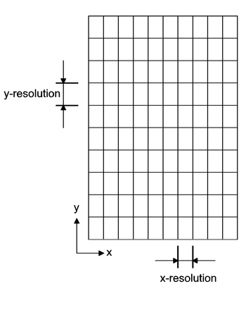
The most common method of archaeological geophysical data acquisition relies on regular grids. They conceptually subdivide the survey area into a raster of many small rectangular cells of equal size (e.g. 0.25 m x 0.5 m) and a measurement is recorded for each cell. In practice this may be realised by walking along lines (e.g. 0.5 m apart) and recording at regular intervals (e.g. every 0.25 m). This geophysics grid then forms the ‘geophysics coordinate system’ to which all measurements are related, either by indicating line and point counts or by referring to it as a Cartesian coordinate system with perpendicular x- and y-axes. Importantly, the resolution of the grid (i.e. its subdivision into small cells) is fixed (Figure 1).

The relationship between positions in this geophysics grid and real location on the ground has to be clearly specified, as explained in the Appendix on Georeferencing Geophysical Data (Appendix 2), otherwise it is impossible to link identified geophysical anomalies to their location on the ground or to results derived from other sources (e.g. aerial photographs).

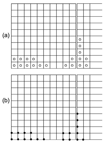
In addition to specifying the particular grid cell at which a measurement was taken the recording position within a grid has to be specified. For example for a 1 m x 1 m grid cell it is important whether the measurement was taken in the centre of the cell (i.e. 50% from the edge in x- and y-direction, Figure 2a) or whether it was recorded in the lower left corner (Figure 2b). Some practitioners for example prefer to walk over tapes that are laid out at regular intervals, which would usually mean that the recording is over the edge of a grid cell, others prefer to walk between tapes, resulting in measurements in the middle of the cell. Some instruments may have similar ‘preferences’: Geoscan magnetometers, for example, are designed such that they assist the operator with regular beeps for every metre walked, including start and finish (resulting in 21 beeps for a 20 m long line) but they actually record the measurements between these beeps in the centre of the grid cells. It is therefore important to note exactly where the readings are located in relation to the grid cells so that a good correlation between data and ground position can be achieved.

It is the intention to always collect data in the exact grid position specified. However, this is seldom possible and the spatial measurement accuracy describes how close, on average, the measurement positions are to the locations indicated by the grid cell. It is useful to estimate this positional accuracy so that the reliability of spatial interpretation can be gauged. The final link between a recorded measurement and its true location on the ground is a combination of this positional accuracy and the georeferencing accuracy of the geophysics grid.

The major advantage of a regular grid is the even coverage of the ground in all locations, which makes comparisons between geophysical anomalies in different locations possible and avoids bias in data interpretation. If data are recorded with varying spatial resolution and then interpolated back to a regular grid (see below), the interpolation algorithm may introduce smooth edges or sharp corners where none really exist. Another advantage of recording on a regular grid is the ease with which the operator can locate their position, just by counting lines and recording points.

However, if a large area is to be surveyed, such counting also becomes difficult and it is therefore very useful to subdivide larger areas into smaller chunks (e.g. of 20 m x 20 m) that occupy only a limited space of the larger geophysics grid. These smaller chunks are given various names by different practitioners, for example by archaeological geophysics instrument manufacturers simply as ‘grids’, by remote sensing experts as ’tiles’ and sometimes as ‘sub grids’. In accordance with Aspinall et al. (2008) we use the term ‘data grids’ in this Guide. In addition to subdividing a large survey area into manageable chunks, which can then again be indexed through row and column counts data grids also have other advantages. Some magnetometers exhibit instrument drift which may not necessarily be constant over time. Monitoring such a drift for each individual data grid therefore allows more efficient processing and correction of this effect. Twin probe earth resistance measurements require the relocation of the remote electrodes when the cable length becomes insufficient for more distant recording positions. Undertaking such a survey over chunks of data grids makes these operations far more efficient. It should also not be underestimated that subdividing a large area greatly helps with the motivation of survey personnel (“only two more grids to go”). Data grids can be named according to the sequence in which they are recorded but if the same data grid is used with different instruments but in a different order (e.g. magnetometers and earth resistances meters) this may become confusing and naming by a combination of letters and numbers (similar to a computer spreadsheet) could be useful to reflect their position in the overall geophysics grid.

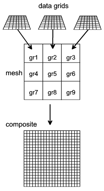
If data acquisition is undertaken over several data grids it is important to record this sequence, for example to monitor an instrument’s drift and later correct for it. Obviously, it is essential to provide clear indications as to where each data grid is located in the overall geophysics grid. This can either be done through a map of the data grids, visualised as a mesh (also referred to as ‘master grid’) or by specifying the x- and y- coordinates of the corners of each data grid. Using this information all recorded measurements from all data grids can be assembled into one large data structure for the whole geophysics grid, often referred to as a ‘composite’ (i.e. data grids + mesh = composite, Figure 3).

Line data

One alternative to the use of a regular grid is the continuous recording of readings while walking along straight lines. In the past systems were designed with analog and continuous recording on mechano-electrical strip charts (Clark 1996). Modern digital instruments have fast continuous digital recording of measurements (e.g. at a rate of 10Hz) or are triggered at selected spatial intervals using an odometer wheel or GNSS/GPS. These data can be represented as continuous line graphs, similar to a spreadsheet graph, or they are re-sampled to a grid with a resolution that is chosen to match the line data as well as possible.

Non-gridded data

Recording the measurements (geophysics data) as well as their location (e.g. using GNSS/GPS or a Total Station) during the survey allows to collect data without a predefined grid. If no further spatial guidance is used (‘random walk’) the resulting data density can be very uneven, covering some areas very densely while in other parts large gaps exist between the walked lines. Guidance systems are now available that show the already covered tracks so that the data collection can be somewhat adjusted.

The resulting data are usually re-sampled in X- and Y- direction to a regular grid so that grid-based processing software can be used for further data enhancement. The shortcomings of individual gridding algorithms should be carefully considered and the mechanisms for filling gaps between data tracks taken into account when interpreting the results.

A different approach is the direct use of these data without re-gridding. Sauerländer et al. (1999) demonstrated that representing such data as a two-dimensional Voronoi diagram is a very effective way of retaining their original spatial properties and visualising the density of data collection.