A variety of computer algorithms are available to improve and enhance the measured geophysical data and they are often all referred to as data processing. However, since some require earlier steps and different metadata it is conceptually clearer if they are subdivided in steps for data improvement, data processing and image processing.

Data improvement

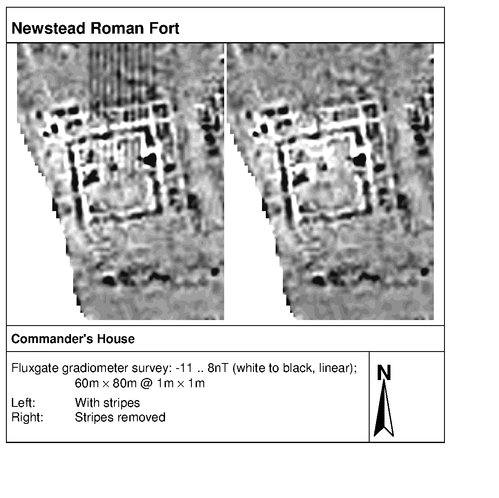
If information on the process of data acquisition is available, some common surveying errors can be rectified with appropriate software. For example, if data were collected on adjacent lines, drift of an instrument’s reference value can often be reduced. Such processing can however only be applied if data are available in a format that reflects the surveying procedure (e.g. if data are saved as separate data grids) and if information on the surveying strategy is given. Data improvement usually is applied to individual data grids as these are the units in which data were collected and hence delimit defects during survey. Typical examples include drift correction, destaggering, destriping (see Figure 4) and grid balancing.

Data processing

Once all data grids have been improved and a seamless composite produced this can be processed to deal with effects of the data and not with defects created during their acquisition. For example, if a very high reading produced by metal debris (fallen from a tractor) creates a magnetometer ‘spike’ across two data grids, the despiking procedure has to be applied after the grids were corrected for drift and been balanced. It is also possible to apply processing algorithms that are pertinent to the geophysical nature of the acquired data, for example using high-pass filtering for earth resistance data over a geological background variation (see Figure 5) or computing a reduction-to-the-pole for magnetometer data.

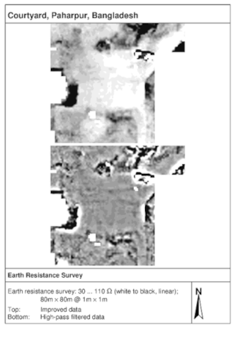
Image processing

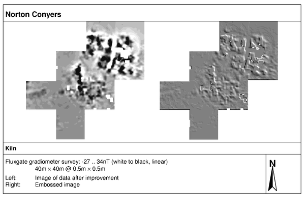
Data are just numbers and have to be visualised to analyse and interpret them. In the past this often took the form of contour diagrams but now greyscale raster images are the most commonly used method. To do this a ‘transfer function’ is used that determines how each data value is converted to a display colour. In this process very high and low values are usually ‘clipped’ (i.e. mapped to the same display colour) and overall the process is irreversible. Once the image pixels are calculated, the real measurement data cannot be reconstructed. This creates problems if subtle information is to be extracted as the range of for example display grey shades (e.g. 0 to 255) is much coarser than the full data range (e.g. -20.05 to +500.07 nT). When data are converted to images for display or file storage important information is therefore lost. Images are extremely useful for evaluating data but they are no replacement for the recorded measurements. These images can only be treated with standard image processing tools that cannot take into account the geophysical nature of the underlying data (see the Guide to Raster Images). Although of little use for geophysical analysis of the data, image processing functions in standard image software (e.g. embossing, see Figure 6) may still be useful to convey relevant information to users.